Protein Function Prediction using LoRA-Relational Graph Neural Networks and Multi-Task Learning
This is my class project for CS224W: Machine Learning on Graphs, done in collaboration with Alec Lessing and Matt Wolff. I won’t go into every detail here, but you can read our in-depth Medium post if you want the full picture!
The task was to predict whether or not a protein possesed a particular functional property. We used AlphaFold 2’s protein structure predictions. Each node in the input graph represents an atom with features consisting of the 3D atom coordinates and the one-hot-encoded atom type. We also augmented these features with cycle counts, in order to surpass the expressivity limitations of the Weisfeiler Leman (WL) isomorphism test.
Structural Feature Augmentation
More precisely, in the naive setting, the feature for node \(i\) is its one-hot-encoded atom type, a number representing the number of protons in the atom. In our dataset, the only atom types are Boron, Carbon, Nitrogen, Sulfur so we use a 4-dimensional one-hot encoding for atom type. To make the graph neural network (GNN) more expressive, the feature for node \(i\) will be augmented by:
\[\mathbf{s}=\begin{bmatrix} diag(A^0)_{i,i} ,\dots, diag(A^{K-1})_{i,i} \end{bmatrix}\in\mathbb{R}^K\]where the \((i,i)\) entry of the diagonal of the \(k\)-th power of the adjacency matrix \(A\) corresponds to the number of \(k\)-length cycles node \(i\) resides in. In fact, in the recent work of Kanatsoulis et al., it was shown that a Graph Isomorphism Network (the most powerful GNN in the class of message-passing GNNs) with such structural initial node features is strictly more powerful than the WL test!
Three-way Classification
We use structural counts, atom types, and coordinates, to make a graph-level 3-way classification of whether a protein (1) contributes to, (2) enables, or (3) does not enable/contribute to a specific function.
Heterogeneous Protein Graph and Relational GAT
We obtain a graph-level embedding for the protein using a graph neural network:
\[\begin{split} &f_{\theta}: \mathbb{R}^{N\times (K+4)} \times \mathbb{R}^{N\times 3} \rightarrow \mathbb{R}^H\\ &\mathbf{p}_{\theta}=f_{\theta}(H, X) \end{split}\]where \(H\in\mathbb{R}^{N\times (K + 4)}\) is the matrix of augmented node features and \(X\in\mathbb{R}^{N\times 3}\) is the matrix of the predicted coordinates for the protein from AlphaFold.
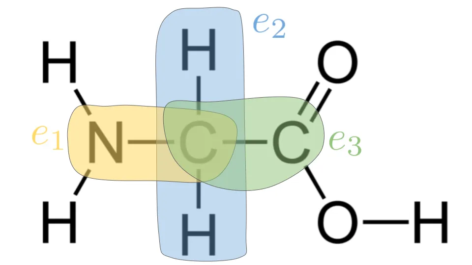
We view the protein graph as a heterogenous graph, whereby (source_atom_type, target_atom_type) is an edge type. In our setting, this is equivalent to a relation type. For instance, in the glycine amino acid molecule shown below, (Carbon, Hydrogen) is distinct from (Carbon, Nitrogen). Intuitively, we should treat the graph as heterogenous so the message-passing GNN can distinguish edge types. In our dataset, there are 16 unique edge types.

As shown in this figure, if we we update the feature representation for the central Carbon atom, we would only perform message passing and aggregation over distinct edge types, namely $e_1$: (C, N), $e_2$: (C, H), $e_3$: (C, C). We use Relational Graph Attention Network (RGAT) to process this heterogenous protein graph structure. We apply a linear transformation to the input features for each relation type \(r\):
\[\begin{split} &H\in\mathbb{R}^{N\times F}\\ &W_1^{(r)}\in\mathbb{R}^{F\times F'}\\ &G^{(r)}=HW_1^{(r)}=\begin{bmatrix}\mathbf{g}_1^{(r)} & \dots & \mathbf{g}_N^{(r)} \end{bmatrix}\in\mathbb{R}^{N\times F'} \end{split}\]Given linear transformations \(W_1^{(r)}\) of type \(r\), we assume that the logits of each relation are independent, given by:
\[E_{ij}^{(r)}=a(\mathbf{g}_i^{(r)}, \mathbf{g}_j^{(r)}, \mathbf{e}_{ij}^{(r)}).\]This denotes the importance of node \(j\)’s representation to that of node \(i\) under relation \(r\). We additionally condition on the edge attribute \(\mathbf{e}_{ij}\), which we will define as the distance between atoms in our application. We chose to use an additive attention mechanism a, whereby we project intermediate representations \(g\) into query and key representations of dimension \(D\) and add them with the projected pair-wise distance edge attribute:
\[\begin{split} &Q^{(r)}, K^{(r)}\in\mathbb{R}^{F'\times D}, W_2^{(r)}\in\mathbb{R}^{D\times 1}\\ &\mathbf{q}_i^{(r)}=g_i^{(r)}Q^{(r)}\in\mathbb{R}^D\\ &\mathbf{k}_i^{(r)}=g_i^{(r)}K^{(r)}\in\mathbb{R}^D\\ &\mathbf{e}_{ij}^{(r)}=||\mathbf{x}_i^{(r)}-\mathbf{x}_j^{(r)}||_2\in\mathbb{R}\\ &E_{ij}^{(r)}=\text{LeakReLU}(q_i^{(r)} + k_j^{(r)} + W_2^{(r)}\mathbf{e}_{ij}^{(r)}). \end{split}\]Then, attention coefficients are computed across neighborhoods, irrespective of the relation - this is known as \(\textit{Across-Relation Graph Attention}\):
\[\begin{split} &\alpha_{i,j}^{(r)}=\text{softmax}_{j,r}(E_{ij}^{(r)})=\frac{\exp(E_{ij}^{(r)})}{\sum_{r'\in\mathcal{R}}\sum_{k\in\mathcal{N}_i^{(r')}}\exp(E_{ik}^{(r')})}\\ &\sum_{r\in\mathcal{R}}\sum_{j\in\mathcal{N}_i^{(r)}}\alpha_{i,j}^{(r)}=1 \end{split}\]where \(\mathcal{N}_i^{(r)}\) represents the neighborhood of \(i\) under relation \(r\). Finally, we aggregate the intermediate representations and apply a non-linear activation:
\[\mathbf{h}_i'=\sigma\left(\sum_{r\in\mathcal{R}}\sum_{j\in\mathcal{N}_i^{(r)}}\alpha_{ij}^{(r)}\mathbf{g}_j^{(r)}\right)\in\mathbb{R}^{N\times F'}.\]Low-Rank Adaptation for Efficient Relational Graph Neural Networks
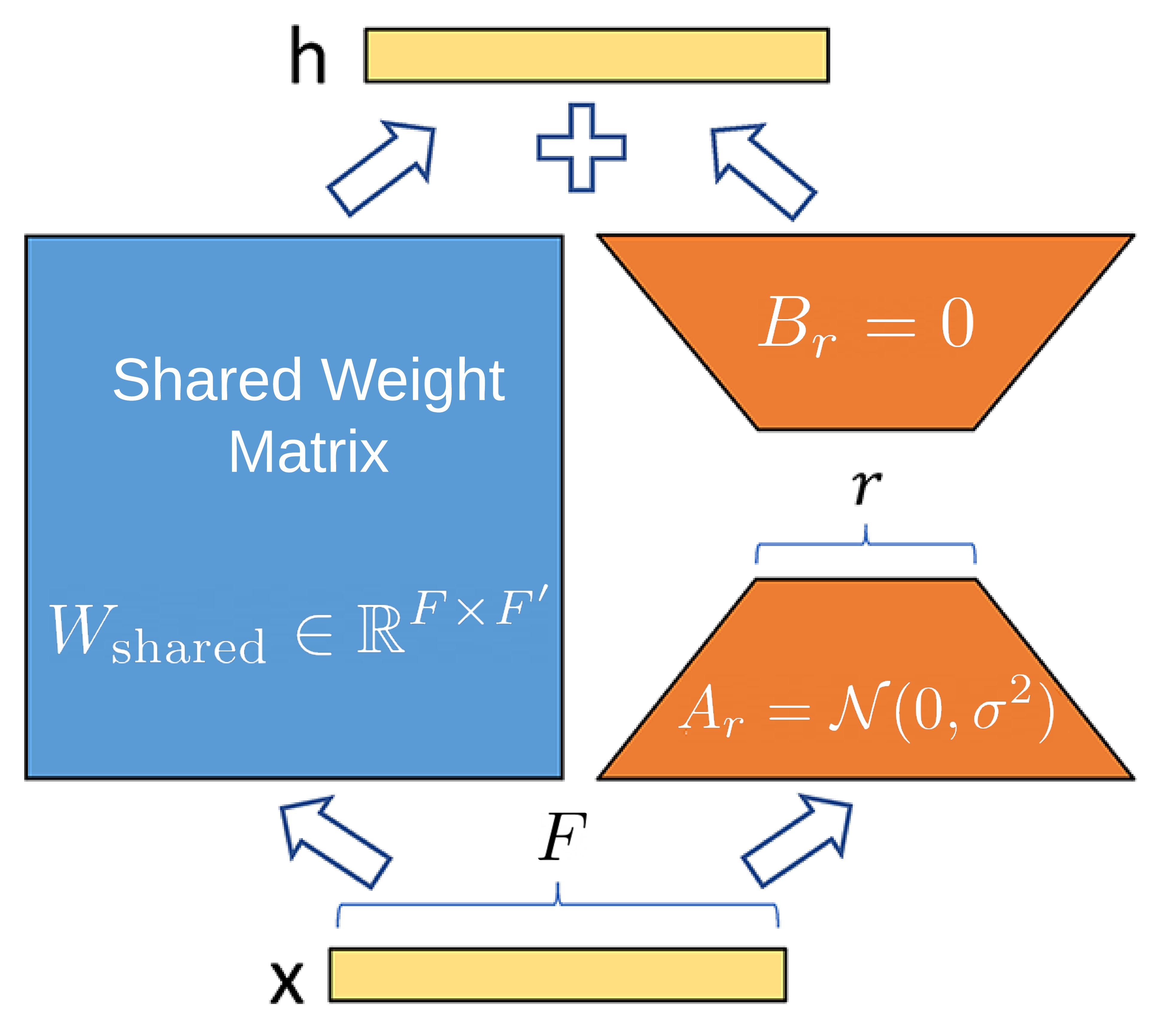
As we have 16 relation types and use a large hidden dimension in our experiments (512), it would be inefficient to maintain a weight matrix W(r) for every type, as described in RGAT. Thus, we propose a decomposition based on Low-Rank Adaptation of Large Language Models [12]. We decomposed W(r) into a shared weight matrix for all relation types and a low-rank decomposition for the relation-specific component. That is: \(W_r=W_{\text{shared}} + A_r B_r\) where \(W_{\text{shared}}\in\mathbb{R}^{F\times F'}\) is a shared weight matrix and \(A_r\in\mathbb{R}^{F\times r}\), \(B_r\in\mathbb{R}^{r\times F'}\) are two low-rank matrices such that \(r<<\min(F, F')\). Concretely, if \(F=512\), \(F'=512\), and \(|\mathcal{R}|=16\), then for all the \(W_r\) matrices, we would require \(16 * 512 * 512 = 4,194,304\) parameters per layer of the RGAT. However, using this proposed LoRA decomposition, if \(r = 5\), we only use \(512 * 512 + 16 * 2 * 512 * 5 = 344,064\), an order of magnitude reduction. As shown in the figure below, following the original LoRA paper, we use random Gaussian initialization for \(A_r\) and zero for \(B_r\).

Pooling Layer
The embeddings of all the nodes in the protein graph are aggregated to obtain a graph-level protein representation. We do so with a global mean pooling layer: \(\mathbf{p}=\frac{1}{N}\sum_{i=1}^N\mathbf{h}_i' \in\mathbb{R}^H\) where \(\mathbf{h}_i'\) is the final layer embedding for atom \(i\).
Multi-task Learning for Protein Functions
At test time, for each protein \(b\), the objective is to predict whether it possesses a randomly sampled function - which we call a \(\textit{task}\). This is a multi-task problem, whereby we hold out proteins during training and, at test time, we perform \(3\)-way classifications for all tasks associated with a protein. Specifically, for each protein \(b\) and atom \(i\), we feed input coordinates \(\mathbf{x}_i\) and features \(\mathbf{h}_i\) to a neural network \(f_{\theta}\) to obtain a \(D\)-dimensional latent protein representation \(\mathbf{p}_{\theta}^{(b)}\). Our dataset consists of \(B\) proteins, with protein embeddings \(\mathbf{p}_{\theta}^{(b)}\), and the corresponding ground-truth label for a task index \(t^{(b)}\). We define a positive dataset, consisting of pairs of a protein embedding and the corresponding labels for the function tasks associated with that protein:
\[\mathcal{D}^+:=\left\{\mathcal{D}_b^+\right\}_{b=1}^B:=\left\{\{(\mathbf{p}_{\theta}^{(b)}, y^{(t^{(b)})})\}_{t^{(b)}\in\mathcal{T}_b^+}\right\}_{b=1}^B\]where \(\mathcal{T}_b^{+}\) is the set of all indices of real tasks for protein \(b\). We also define a negative dataset, consisting of pairs of a protein embedding and the labels for randomly sampled “negative” function tasks that we generated to balance the positive dataset:
\[\mathcal{D}^-:=\left\{\mathcal{D}_b^-\right\}_{b=1}^B:=\left\{\{(\mathbf{p}_{\theta}^{(b)}, y^{(t^{(b)})})\}_{t^{(b)}\in\mathcal{T}_b^-}\right\}_{b=1}^B\]where \(\mathcal{T}_b^{-}\) denotes indices corresponding to the fake tasks for protein \(b\). Thus, for a protein \(b\), we sample a task \(t^{(b)}\) and compute its embedding with a look-up embedding table:
\[\mathbf{t}^{(b)}=\text{Embed}_{\psi}(t^{(b)})\in\mathbb{R}^{E}\]We also obtain its latent protein embedding from its features and coordinates:
\[\mathbf{p}_{\theta}^{(b)}=f_{\theta}(H^{(b)},X^{(b)})\in\mathbb{R}^{H}\]Finally, we use an MLP with a softmax applied to its logits to condition our classification on the task embedding and obtain the discrete probability distribution that protein \(b\) contributes to, enables or does not enable/contribute to protein function with task index \(t^{(b)}\):
\[\begin{split} &g_{\phi}:\mathbb{R}^{E}\times \mathbb{R}^{H}\to[0,1]^3\\ &\hat{y}^{(t^{(b)})}=g_{\phi}(\mathbf{t}^{(b)}, \mathbf{p}^{(b)}). \end{split}\]Hence, we will minimize the following cross-entropy objective:
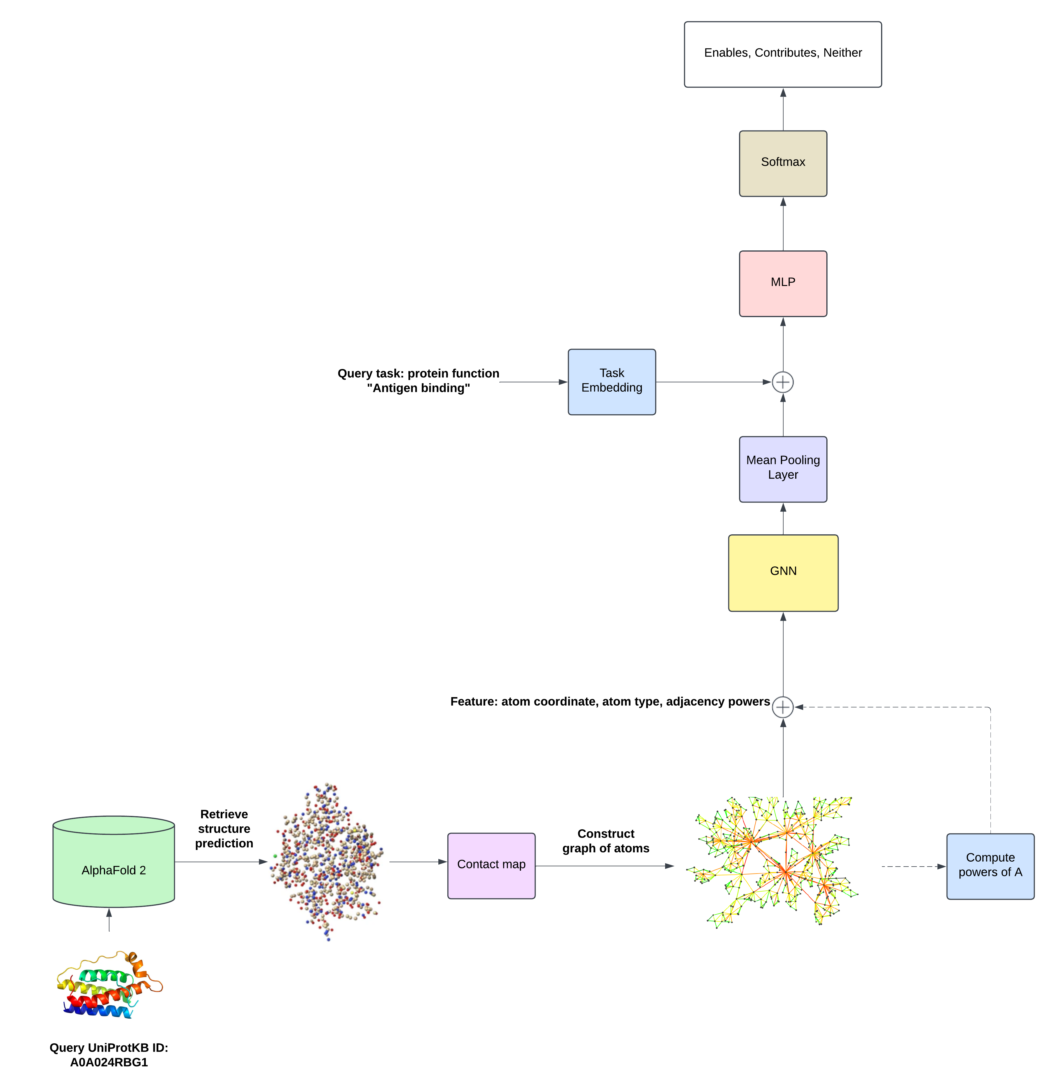
\[\min_{\psi,\theta,\phi}\sum_{b=1}^B \sum_{\left(\mathbf{p}_{\theta}^{(b)}, y^{(t^{(b)})}\right)\in\mathcal{D}_b^+\cup\mathcal{D}_b^-}\mathcal{H}\left(y^{(t^{(b)})}, g_{\phi}\Big(\text{Embed}_{\psi}(t^{(b)}), \mathbf{p}_{\theta}^{(b)}\Big)\right)\]via a finite-sample approximation using mini-batch stochastic gradient descent. The complete architecture for FuncE GNN is illustrated below.
